Types and Programming Languages
17 Jan 2015Note: This is a summary of the book Types and Programming Languages.
- Operational Semantics
- Lambda Calculus
- Simply Typed Lambda Calculus
- Reference Type
- Universal Type
- Type Reconstruction
- Existential Type
- Recursive Type
- Subtyping
- Object
- Featherweight Java
- Bounded Quantification
- Kinding and Higher-Order Polymorphism
- Higher-Order Bounded Polymorphism
Operational Semantics
An abstract machine consists of:
- a set of states
- a transition relation on states
A state records all the information in the machine at a given moment.
A normal form is a term that cannot be evaluated any further.
Lambda Calculus
Lambda calculus is the foundation for many programming languages. It’s more widely used than the Turing machine model in programming language studies due to its nice mathematical properties.
- Turing complete
- Everything is a function
- variables always denote functions
- function always take functions as parameters
Syntactically, “everything is a function” doesn’t work, we need variables. Ontologically it works, all closed lambda terms denote standalone functions.
There are several evaluation strategies for lambda calculus, call by value is the most widely used.
- Call by value(most languages)
- Call by name(Haskell)
- Normal order(left-most/outer-most)
- Full-beta
Call by value specification:
SYNTAX

t ::=                      terms
      x                      variable
      λx.t                   abstraction
      t t                    application


EVALUATION

(λx.t) v ⟶  [x ⟼ v]t        (E-AppAbs)

   t1  ⟶  t1'
------------------           (E-App1)
t1 t2  ⟶  t1' t2

   t2  ⟶  t2'
------------------           (E-App2)
v1 t2  ⟶  v1 t2'
We can represent numbers, booleans, pairs, recursion functions, etc based on lambda calculus:
tru = λt. λf. t
fls = λt. λf. f

and = λb. λc. b c fls
or = λb. λc. b tru c
not = λb. b fls tru

pair = λf.λs.λb. b f s
fst = λp. p tru
snd = λp. p fls


0 = λs. λz. z
1 = λs. λz.s z
2 = λs. λz.s (s z)
3 = λs. λz.s (s (s z))
...

scc= λn. λs. λz.s(n s z)
plus= λm. λn. λs. λz.ms(n s z)
times = λm. λn. λs. λz. m (n s) z
power = λm. λn. n (times m m)

fix = λf. (λx. f (λy. x x y)) (λx. f (λy. x x y))
fact = fix ( λfct. λn. if iszero n then 1 else n * (fct (pred n)) )
behavioral equivalence
Two lambda terms are observationally equivalent if they both diverge or reduce to a value.
Two lambda terms are behaviorally equivalent if they are observationally equivalent to all possible applications.
Simply Typed Lambda Calculus
Typing helps exclude certain bad terms – sometimes with the price of excluding some meaningful terms.
Structural Types VS. Nominal Types
For structural type systems, what matters about a type (for typing, subtyping, etc.) is just its structure. Names are just convenient (but inessential) abbreviations.
For nominal type systems:
- Types are always named.
- Typechecker mostly manipulates names, not structures.
- Subtyping is declared explicitly by programmer.
Structural types are simpler, cleaner, and more elegant, while nominal types make recursive types easier, make typechecking more efficient, and make it possible to use type name in runtime.
Type Safety
A type relation is sound if it satisfied preservation and progress.
- preservation. If t:T and t -> t’, then t’:T.
- progress. If t:T, either t is a value or there exists t’ such that t -> t’.
To define and verify a type system, you must:
- Define types
- Specify typing rules
- Prove soundness: progress and preservation
Specification of STLC
The main usage of types is to exclude invalid terms. Type checking happens at compile time, they have nothing to do with evaluation, thus can be erased before evaluation.
The pure STLC is not interesting, as it only has one type ->. Variants of STLC are augmented with primary types like Bool or Nat.
SYNTAX

t ::=                      terms
      x                      variable
      λx:T.t                 abstraction
      t t                    application
      true                   constant true
      false                  constant false
      if t then t else t     conditional

v ::=                      values
      x.t                    abstraction value
      true                   true value
      false                  false value

T ::=                      types
      Bool                   type of booleans
      T → T                  types of functions

Γ ::=                          contexts
      ∅                          empty context
      Γ, x:T                     term variable binding

EVALUATION

(λx.t) v ⟶  [x ⟼ v]t        (E-AppAbs)

   t1  ⟶  t1'
------------------           (E-App1)
t1 t2  ⟶  t1' t2

   t2  ⟶  t2'
------------------           (E-App2)
v1 t2  ⟶  v1 t2'

TYPING

true : Bool                  (T-True)

false : Bool                 (T-False)

Γ ⊢ t1: Bool, t2: T, t3: T
----------------------------   (T-If)
Γ ⊢ if t1 then t2 else t3: T

Γ, x: T1 ⊢ t: T2
---------------------          (T-Abs)
Γ ⊢ λx:T1.t : T1 → T2

 x:T ∈ Γ
----------                     (T-Var)
Γ ⊢ x : T

Γ ⊢ t1: T → T', t2: T
-----------------------        (T-App)
  Γ ⊢ t1 t2: T
Ascription
SYNTAX:

t ::= ...                       terms
      t as T                      ascription


EVALUATION

v1 as T ⟶  v1                   (E-Ascribe)

     t1 ⟶  t1'
--------------------            (E-Ascribe1)
t1 as T ⟶  t1' as T

TYPING

Γ ⊢ t1: T
--------------------            (T-Ascribe)
Γ ⊢ t1 as T: T
Let
SYNTAX

t ::= ...                        terms
      let x=t in                   let binding


EVALUATION

let x=v1 in t2 ⟶ [x1 ⟼ v1]t2               (E-LetV)

            t1  ⟶  t1'
-----------------------------------          (E-Let)
let x=t1 in t2  ⟶  let x=t1' in t2

TYPING

Γ ⊢ t1: T1, Γ, x: T1 ⊢ t2: T2
----------------------------------           (T-Let)
      Γ ⊢ let x=t1 in t2: T2
Tuple
SYNTAX

t ::= ...                                    terms
      { t(i) | i ∈ 1..n }                      tuple
      t.i                                      projection

v ::= ...                                    values
      { v(i) | i ∈ 1..n }                      tuple value

T ::= ...                                    types
      { T(i) | i ∈ 1..n }                      tuple type


EVALUATION

{ v(i) | i ∈ 1..n }.j  ⟶  v(j)              (E-ProjTuple)

  t1 ⟶  t1'
-------------                                (E-Proj)
t1.j ⟶  t1'.j

             t(j)  ⟶  t'(j)
---------------------------------------------   (E-Tuple)
{ v(i), t(j), t(k)  | i ∈ 1..j-1, k ∈ j+1..n }
⟶
{ v(i), t'(j), t(k) | i ∈ 1..j-1, k ∈ j+1..n }


TYPING

TYPING

   for each i   Γ ⊢ t(i) : T(i)
---------------------------------------------   (T-Tuple)
Γ ⊢ { t(i) | i ∈ 1..n }: { T(i) | i ∈ 1..n }

Γ ⊢ t1: { T(i) | i ∈ 1..n }
------------------------------                  (T-Proj)
      Γ ⊢ t1.j : T(j)
Record
SYNTAX

t ::= ...
      { l(i) = t(i) | i ∈ 1..n }              record
      t.l                                     projection

v ::= ...
      { l(i) = v(i) | i ∈ 1..n }              record value

T ::= ...
      { l(i):T(i) | i ∈ 1..n }                type of records


EVALUATION

{ l(i) = v(i) | i ∈ 1..n }.l(j)  ⟶  v(j)     (E-ProjRcd)

   t1 ⟶ t1'
-----------------                             (E-Proj)
 t1.l   ⟶ t1'.l

           t(j)  ⟶  t'(j)
------------------------------------------    (E-Rcd)
{ l(i) = v(i), l(j) = t(j), l(k) = t(k)
  | i ∈ 1..j-1, k ∈ j+1..n }
⟶
{ l(i) = v(i), l(j) = t'(j), l(k) = t(k)
  | i ∈ 1..j-1, k ∈ j+1..n }


TYPING

             for each i   Γ ⊢ t(i) : T(i)
-----------------------------------------------------------   (T-Rcd)
Γ ⊢ { l(i) = t(i) | i ∈ 1..n }: { l(i) : T(i) | i ∈ 1..n }

Γ ⊢ t1: { l(i) : T(i) | i ∈ 1..n }
----------------------------------                            (T-Proj)
      Γ ⊢ t1.l(j) : T(j)
Sum
SYNTAX

t ::= ...
      inl t as T
      inr t as T

v ::= ...
      inl v as T
      inr v as T


TYPING

       Γ ⊢ t1 : T1
---------------------------       (T-Inl)
Γ ⊢ inl t1 as T1+T2 : T1+T2

       Γ ⊢ t1 : T1
---------------------------       (T-Inr)
Γ ⊢ inr t1 as T1+T2 : T1+T2


EVALUATION

case (inl v0 as T0) of inl x1⟹t1 | inr x2⟹t2  ⟶ [x1 ⟼ v0]t1     (E-CaseInl)

case (inr v0 as T0) of inl x1⟹t1 | inr x2⟹t2  ⟶ [x2 ⟼ v0]t2     (E-CaseInr)

           t1 -> t1'
-------------------------------      (E-Inl)
inl t1 as T2  ⟶  inl t1' as T2

           t1 -> t1'
-------------------------------      (E-Inr)
inr t1 as T2  ⟶  inr t1' as T2
Variants
SYNTAX:

t ::= ...                               Terms
      < l=t > as T                        tagging
      case t of < l(i) = x(i) > ⟹ t(i)   case

T ::= ...                               Types
      < l(i): T(i) | i ∈ 1..n >           types of variants


EVALUATION

case (< l(j) = v(j) > as T) of          (E-CaseVariant)
  < l(1) = x(1) > ⟹ t(1)
  < l(2) = x(2) > ⟹ t(2)
  ...
⟶
[x(j) ⟼ v(j)]t(j)

      t0  ⟶  t0'
-------------------------               (E-Case)
case t0 of
  < l(1) = x(1) > ⟹ t(1)
  < l(2) = x(2) > ⟹ t(2)
  ...
⟶
case t0' of
  < l(1) = x(1) > ⟹ t(1)
  < l(2) = x(2) > ⟹ t(2)
  ...

t(i)  ⟶  t'(i)
---------------------                   (E-Variant)
< l(i)=t(i) > as T
⟶
< l(i)=t'(i) > as T


TYPING

                Γ ⊢ t(j) : T(j)
-----------------------------------------------      (T-Variant)
Γ ⊢ < l(i)=t(i) > as < l(i): T(i) | i ∈ 1..n >
  : < l(i): T(i) | i ∈ 1..n >

    Γ ⊢ t0: < l(i): T(i) | i ∈ 1..n >
   for each i Γ, x(i): T(i) ⊢ t(j) : T
-------------------------------------------          (T-Case)
Γ ⊢ case t0 of
      < l(1) = x(1) > ⟹ t(1)
      < l(2) = x(2) > ⟹ t(2)
      ...
  : T
Example:
  Addr = < physical:PhysicalAddr, virtual:VirtualAddr >;

a = < physical=pa > as Addr;

getName =  λa:Addr.
case a of
     < physical=x > => x.firstlast
   | < virtual=y >  => y.name
Options and enumerations are special cases of variants.
Recursion
In STLC, all terms terminate. It’s impossible to implement recursion using the fix combinator as in untyped lambda calculus. However, it’s possible to introduce the fix combinator into the language to restore the ability to do recursive computation.
SYNTAX

t ::= ...                      terms
      fix t                      fix point of t


EVALUATION

fix (λx:T1. t2)
⟶                             (E-FixBeta)
[x ⟼ (fix (λx:T1. t2))]t2


   t ⟶  t'
---------------                (E-Fix)
fix t ⟶  fix t'


TYPING

Γ ⊢ t: T → T
-------------                  (T-Fix)
Γ ⊢ fix t: T
To make the usage of fix combinator easier, the syntactic sugar letrec is introduced:
letrec x:T1=t1 in t2
⟹
let x = fix (λx:T1.t1) in t2

letrec iseven : Nat!Bool =
  λx:Nat.
    if iszero x then true
    else if iszero (pred x) then false
    else iseven (pred (pred x))
in
  iseven 7
Reference Type
Mutable state is a popular programming model. How can we model mutable states? Mutable states doesn’t only bring changes to the model, but also things that don’t change. As change is only meaningful if it can happen to something that doesn’t change. A common approach to model mutable state is to represent the unchanged as a location or cell, so that the changes can be modeled as the things that the location or cell holds.
Though mutable state makes a lot of things natural and simple, it introduces the problem of aliasing. With the introduction of storage cells, it’s possible that there are multiple references to the same cell in different places of a program under different names. Without some careful coordination or well-defined protocol, this could lead to a chaos.
Another issue with mutable state is that now the order of evaluation matters. Lazy evaluation doesn’t make sense in the context of mutable state.
SYNTAX

t ::= ...                     terms
      ref t                     reference creation
      !t                        dereference
      t:=t                      assignment
      l                         store location

v ::= ...                     values
      l                         store location

EVALUATION

     t1 | μ  ⟶  t1' | μ'
-------------------------------         (E-Assign1)
t1 := t2 | μ ⟶  t1' := t2 | μ'

     t2 | μ  ⟶  t2' | μ'
-------------------------------         (E-Assign2)
v1 := t2 | μ ⟶  v1 := t2' | μ'

l := v2 | μ   ⟶   unit | [l ⟼ v2]μ    (E-Assign)

    t | μ  ⟶  t' | μ'
-------------------------               (E-Ref)
ref t | μ  ⟶  ref t' | μ'

        l ∉ dom(μ)
----------------------------            (E-RefV)
ref v | μ ⟶ l | (μ, l ⟼ v)

 t | μ  ⟶  t' | μ'
--------------------                    (E-DeRef)
!t | μ  ⟶  !t' | μ'

    μ(l) = v
-----------------                       (E-DerefLoc)
!l | μ  ⟶  v | μ

(λx.t) v | μ  ⟶  [x ⟼ v]t | μ          (E-AppAbs)

    t1 | μ ⟶  t1' | μ'
--------------------------              (E-App1)
t1 t2 | μ  ⟶  t1' t2 | μ'

    t2 | μ ⟶  t2' | μ'
--------------------------              (E-App2)
v1 t2 | μ  ⟶  v1 t2' | μ'


TYPING

     Σ(l) = T
-------------------                     (T-Loc)
Γ | Σ  ⊢  l: Ref T

    Γ|Σ ⊢ t: T
----------------------                  (T-Ref)
Γ|Σ ⊢ ref t: Ref T

Γ|Σ ⊢ t: Ref T
--------------                          (T-Deref)
Γ|Σ ⊢ !t: T

Γ|Σ ⊢ t1: Ref T    Γ|Σ ⊢ t2: Ref T
-----------------------------------     (T-Assign)
Γ|Σ ⊢ t1:=t2: Unit
Note that in the above, we augment each evaluation rule with the evaluation environment μ in order to track state of the program. In the typing rules, the store typing Σ is introduced to speed up type checking, instead of computing it from ref t expressions.
Universal Type
Universal type can model polymorphism in programming languages. The logic theory behind universal type is System F, which is introduced by Jean-Yves Girard (1972). It is also sometimes called the second-order lambda-calculus, because it corresponds, via the Curry-Howard correspondence, to second-order intuitionistic logic, which allows quantification not only over individuals [terms], but also over predicates [types].
SYNTAX

t ::= ...                terms
      λX.t                 type abstraction
      t [T]                type application

v ::= ...                values
      λX.t                 type abstraction value

T ::= ...                types
      X                    type variable
      ∀X.T                 universal type

Γ ::=                    contexts
      ∅                    empty context
      Γ, x:T               term variable binding
      Γ, X                 type variable binding

EVALUATION

     t1 ⟶  t1'
-------------------              (E-TApp)
t1 [T2] ⟶  t1' [T2]

(λX.t) [T] ⟶  [X ⟼ T]t          (E-TappTabs)


TYPING

Γ , X ⊢ t : T
----------------                 (T-TAbs)
Γ ⊢ λX.t : ∀X.T

     Γ ⊢ t : ∀X.T
-------------------------        (T-TApp)
 Γ ⊢ t [T1] : [X ⟼ T1]T
In simply typed lambda calculus, there’s no way to type the term “λx. x x”. However, it’s possible in System F:
term: λx:∀X.X→X. x [∀X.X→X] x
type: (∀X. X→X) → (∀X. X → X)
It’s possible to type Church encodings in System F:
CBool = ∀X.X→X→X
true  = λX. λt:X. λf:X. t
false = λX. λt:X. λf:X. f

CNat = ∀X. (X→X) → X → X
0 = λX. λs:X→X. λz:X. z
1 = λX. λs:X→X. λz:X. s z
Type Reconstruction
- Type checking: Given Γ, t and T, check whether Γ ⊢ t : T.
- Type reconstruction: Given Γ and t, find a type T such that Γ ⊢ t : T.
In general, a type reconstruction algorithm A assigns to an environment !and a term t a set of types 𝒜(Γ, t).
The algorithm is sound if for every type T ∈ 𝒜(Γ, t) we can prove the judgment Γ ⊢ t : T.
The algorithm is complete if for every provable judgment Γ ⊢ t : T we have that T ∈ 𝒜(Γ, t).
Type reconstruction with subtyping and universal types are difficult. Here we only concern us with simple types. The type reconstruction process first generates constraint equations from terms, then use the unification algorithm to solve the equations.
Following are the rules for generating constraint equations:
x: T ∈ Γ
--------------              (CT-VAR)
Γ ⊢ x: T |∅ {}

Γ, x:T1 ⊢ t2: T2 |𝓍 C
-------------------------   (CT-Abs)
Γ ⊢ λx:T1.t2 : T1→T2 |𝓍 C

Γ ⊢ t1 : T1 |𝓍1 C1     Γ ⊢ t2 : T2 |𝓍2 C2
𝓍1 ∩ 𝓍2 = 𝓍1 ∩ FV(T2) = 𝓍2 ∩ FV(T1) = ∅
X ∉ 𝓍1, 𝓍2, T1, T2, C1, C2, Γ, t1, or t2
C′ = C1 ∪ C2 ∪ {T1 = T2→X}
-----------------------------------------  (CT-App)
Γ ⊢ t1 t2 : X |𝓍1 ∪ 𝓍2 ∪ {X} C′

Γ ⊢ true : Bool |∅ {}                  (CT-True)

Γ ⊢ false : Bool |∅ {}                 (CT-False)

Γ ⊢ t1 : T1 |𝓍1 C1
Γ ⊢ t2 : T2 |𝓍2 C2
Γ ⊢ t3 : T3 |𝓍3 C3
𝓍1, 𝓍2, 𝓍3 nonoverlapping
C′ = C1 ∪ C2 ∪ C3 ∪ {T1 = Bool, T2 = T3}
-----------------------------------------------   (CT-If)
Γ ⊢ if t1 then t2 else t3 : T2 |𝓍1 ∪ 𝓍2 ∪ 𝓍3 C′
The unification algorithm is due to Robinson(1965), its usage in type reconstruction is due to Hindley(1969) and Milner (1978).
unify(C) = if C = ∅, then []
           else let {S = T} ∪ C′ = C in
                if S = T
                   then unify(C′)
                else if S = X and X ∉ FV(T)
                  then unify([X ⟼ T]C′) ◦ [X ⟼ T]
                else if T = X and X ∉ FV(S)
                  then unify([X ⟼ S]C′) ◦ [X ⟼ S]
                else if S = S1→S2 and T = T1→T2
                  then unify(C′ ∪ {S1 = T1, S2 = T2})
                else
                  fail
Type reconstruction with universal type is hard. However, type reconstruction for a fragment of System F has been successfully implemented in ML by Milner(1978) under the name let-polymorphism.
The essence of let-polymorphism is to allow multiple different type bindings to the same function. This idea can be easily implemented as follows:
Γ ⊢ [x ⟼ t1]t2 : T2      Γ ⊢ t1 : T1
-------------------------------------     (T-LetPoly)
Γ ⊢ let x=t1 in t2 : T2
However, if there’re many occurrences of x in t1, the type checker would need to do a lot of duplicate work.
A more efficient approach is to bind x to a type scheme, and instantiate the type scheme in each usage of x.
Existential Type
Existential type provides an elegant foundation for data abstraction and information hiding. Existential type corresponds to the existential quantification in logic.
SYNTAX

t ::= ...                terms
      {*T,t} as T          packing
      let {X,x}=t in t     unpacking

v ::= ...                values
      {*T,v} as T          package value

T ::= ...                types
      ∃X.T                 existential type


EVALUATION

let {X,x}=({*T11,v12} as T1) in t2      (E-UnpackPack)
⟶ [X ⟼ T11][x ⟼ v12]t2

              t ⟶  t'
-------------------------------------   (E-Pack)
{*T11, t} as T1  ⟶  {*T11, t'} as T1

              t1 ⟶  t1'
-------------------------------------   (E-Unpack)
       let {X,x}=t1 in t2
    ⟶ let {X,x}=t1' in t2


TYPING

      Γ ⊢ t2 : [X ⟼ U]T2
-------------------------------         (T-Pack)
  Γ ⊢ {*U,t2} as ∃X.T2: ∃X.T2


Γ ⊢ t1 : ∃X.T12    Γ, X, x:T12 ⊢ t2 : T2
----------------------------------------             (T-Unpack)
    Γ ⊢ let {X,x}=t1 in t2 : T2
Special notes in TAPL(Chapter 24):
(1) In the rule T-Unpack, the type variable X appears in the context in which t2’s type is calculated, but does not appear in the context of the rule’s conclusion. This means that the result type T2 cannot contain X free, since any free occurrences of X will be out of scope in the conclusion.
(2) In the rule T-Pack, the type U doesn’t appear in the type signature. It means that packages with different hidden representation types can inhabit the same existential type.
Following is an example of information hiding based on existential type.
ADT counter =
  type Counter
  representation Nat
  signature
    new : Counter,
    get : Counter→Nat,
    inc : Counter→Counter;
  operations
    new = 1,
    get = λi:Nat. i,
    inc = λi:Nat. succ(i)

counter.get (counter.inc counter.new)
The code above can be encoded as follows:
counterADT =
  {*Nat,
    { new = 1,
      get = λi:Nat. i,
      inc = λi:Nat. succ(i) } }
  as ∃Counter.
       { new: Counter,
         get: Counter→Nat,
         inc: Counter→Counter } };

let {Counter,counter} = counterADT in
    counter.get (counter.inc counter.new);
It’s possible to encode existential type in universal type:
∃X.T   =   ∀Y. (∀X. T→Y) → Y

{*S,t} as ∃X.T   =    λY. λf:(∀X.T→Y). f [S] t

let {X,x}=t1 in t2   =    t1 [T2] (λX. λx:T11. t2)
Recursive Type
Recursive types are everywhere, lists and trees are the most common. Ideally, we can define a recursive type NatList as follows:
NatList = <nil:Unit, cons:{Nat,NatList}>
If we’re working with nominal types, then everything is simple and straight-forward. If we limit ourself to structural types, then we have to eliminate the names in the type:
NatList = μX. <nil:Unit, cons:{Nat,X}>
There are generally two approaches to recursive type depending on how they answer following question:
What is the relation between the type μX.T and its one-step unfolding?
For example, what is the relation between NatList and < nil:Unit,cons:{Nat,NatList} >?
- The equi-recursive approach takes these two type expressions as definitionally equal
- The iso-recursive approach takes a recursive type and its unfolding as different, but isomorphic
In a system with iso-recursive types, we have to introduce, for each recursive type μX.T, a pair of functions:
unfold[μX.T] : μX.T → [X ⟼ μX.T] T
fold[μX.T] : [X ⟼ μX.T] T → μX.T
Both approaches are widely used in theoretical studies and practical language design. The equi-recursive approach is more intuitive but difficult to work with bounded quantification and type operators. The iso-recursive approach is heavier in notation, but in practical languages they can be done implicitly by the compiler.
The specification for iso-recursive types (λμ) is listed below:
SYNTAX

t ::= ...                     terms
      fold [T] t                folding
      unfold [T] t              unfolding

v ::= ...                     values
      fold [T] v                folding

T ::= ...                     types
      X                         type variable
      μX.T                      recursive type


EVALUATION

unfold [T] (fold [T] v) ⟶  v     (E-UnfldFld)

         t ⟶  t'
-------------------------        (E-Fld)
fold [T] t ⟶  fold [T] t'

         t ⟶  t'
-----------------------------    (E-Unfld)
unfold [T] t ⟶  unfold [T] t'


TYPING

U = μX.T1    Γ ⊢ t1:[X ⟼ U]T1
------------------------------   (T-Fld)
     Γ ⊢ fold [U] t1 : U

    U = μX.T1    Γ ⊢ t1:U
------------------------------   (T-Unfld)
Γ ⊢ unfold [U] t1 : [X ⟼ U]T1
Subtyping
Why we need subtyping? See the example below:
(λr:{x:Nat}. r.x) {x=0,y=1}
The term doesn’t type check, however we would like it to type check.
SUBTYPING

Γ ⊢  t : S    S <: T
---------------------   (T-Sub)
     Γ ⊢ t : T

S <: S                 (S-Refl)

S <: U     U <: T
------------------      (S-Trans)
      S <: T

{l(i):T(i) | i ∈ 1..n+k} <: {l(i):T(i) | i ∈ 1..n}     (S-RcdWidth)

               for each i Si <: Ti
---------------------------------------------------     (S-RcdDepth)
{l(i):S(i) | i ∈ 1..n}  <:  {l(i):T(i) | i ∈ 1..n}

{k(j):S(j) | j ∈ 1..n} is a permutation of {l(i):T(i) | i ∈ 1..n}
-----------------------------------------------------------------  (S-RcdPerm)
     {k(j):S(j) | j ∈ 1..n}  <:  {l(i):T(i) | i ∈ 1..n}

T1 <: S1     S2 <: T2
-----------------------     (S-Arrow)
  S1 → S2 <: T1 → T2

S <: Top                   (S-Top)
We can also introduce a bottom type Bot in addition to the top type Top, to make the typing relation a lattice. Note that in the S-Arrow rule, the parameter is contra-variant, while the return value is covariant.
The subtype relation in the above is structural: that’s to decide whether S is a subtype of T by examining the structure of S and T. In real world, most languages uses nominal typing. Nominal typing makes recursive types easier, while structural typing is more flexible.
Ref is neither covariant nor contra-variant. That’s the same with Array due to side effects. Java makes Array covariant, which is a mistake in design!
One technique to make Ref work with subtyping is to split its type for read and write, and make read covariant, make write contra-variant.
The intricacy related to reference is caused by the ability to change the type of the cell during execution, similar to the problem in universal type.
Object
Most of class-based object-oriented programming features can be represented with STLC with extensions like reference, records, recursion and subtyping. We’ll show how to represent following object features:
- dynamic dispatch
- encapsulation of state
- inheritance
- this
- super
Encapsulation of State
// Java
class Counter {
  protected int x = 1; // Hidden state
  int get() { return x; }
  void inc() { x++; }
}

void inc3(Counter c) {
  c.inc(); c.inc(); c.inc();
}

// STLC
Counter c = new Counter();
inc3(c);
inc3(c);
c.get();

newCounter =
  λ_:Unit. let r = {x=ref 1} in
     { get = λ_:Unit. !(r.x),
       inc = λ_:Unit. r.x:=succ(!(r.x)) };
Note that encapsulation of state is a form of information hiding. A different approach of information hiding is Abstract Data Type(ADT).
An ADT comprises:
- A hidden representation type X
- A collection of operations for creating and manipulating elements of type X.
The theory behind ADT is existential type. In the OO community, the term “abstract data type” is used as a synonym for “object type”, this usage is very different from its standard usage in academics.
Subtyping and Inheritance
// Java
class Counter {
  protected int x = 1;
  int get() { return x; }
  void inc() { x++; }
}

class ResetCounter extends Counter {
  void reset() { x = 1; }
}

class BackupCounter extends ResetCounter {
  protected int b = 1;
  void backup() { b = x; }
  void reset() { x = b; }
}

// STLC

counterClass =
  λr:CounterRep.
     { get = λ_:Unit. !(r.x),
       inc = λ_:Unit. r.x:=succ(!(r.x)) };

newCounter =
  λ_:Unit. let r = {x=ref 1}
           in counterClass r;

resetCounterClass =
  λr:CounterRep.
    let super = counterClass r in
      { get = super.get,
        inc = super.inc,
        reset = λ_:Unit. r.x:=1 };

newResetCounter =
  λ_:Unit. let r = { x=ref 1 } in resetCounterClass r;

BackupCounter = { get:Unit→Nat, inc:Unit→Unit,
                  reset:Unit→Unit, backup: Unit→Unit };

BackupCounterRep = { x: Ref Nat, b: Ref Nat };

backupCounterClass =
  λr:BackupCounterRep.
    let super = resetCounterClass r
    in
        { get = super.get,
          inc = super.inc,
          reset = λ_:Unit. r.x:=!(r.b),
          backup = λ_:Unit. r.b:=!(r.x) }
this
In Java, we can call between class methods:
class SetCounter {
  protected int x = 0;
  int get () { return x; }
  void set (int i) { x = i; }
  void inc () { this.set( this.get() + 1 ); }
}
First try:
setCounterClass =
  λr:CounterRep.
    fix
      (λthis: SetCounter.
        { get = λ_:Unit. !(r.x),
          set = λi:Nat. r.x:=i,
          inc = λ_:Unit. this.set (succ (this.get unit)) });
The problem with the implementation above is that the binding of this is closed. However, most OO languages support late binding of this, also known as open recursion through this. Open recursion through this allows the methods of a superclass to call the methods of a subclass, even though the subclass does not exist when the superclass is being defined.
We can solve the problem by moving fix out of setCounterClass to newSetCounter.
setCounterClass =
  λr:CounterRep.
    λthis: SetCounter.
      { get = λ_:Unit. !(r.x),
        set = λi:Nat. r.x:=i,
        inc = λ_:Unit. this.set (succ(this.get unit)) }

newSetCounter =
  λ_:Unit. let r = {x=ref 1}
           in fix (setCounterClass r)

InstrCounterRep = {x: Ref Nat, a: Ref Nat}

InstrCounter = { get:Unit→Nat, set:Nat→Unit,
                 inc:Unit→Unit, accesses:Unit→Nat}

instrCounterClass =
  λr:InstrCounterRep.
    λthis: InstrCounter.
      let super = setCounterClass r this in
        { get = super.get,
          set = λi:Nat. (r.a:=succ(!(r.a)); super.set i),
          inc = super.inc,
          accesses = λ_:Unit. !(r.a) }

newInstrCounter =
  λ_:Unit. let r = {x=ref 1, a=ref 0} in
           fix (instrCounterClass r)
A problem with the version above is that newInstrCounter unit will diverge – we’re using this too early in creating super. An inelegant solution to the problem is to delay the usage of this in λ_:Unit t.
setCounterClass =
  λr:CounterRep.
    λthis: Unit→SetCounter.
      λ_:Unit.
        { get = λ_:Unit. !(r.x),
          set = λi:Nat. r.x:=i,
          inc = λ_:Unit. (this unit).set(succ((this unit).get unit)) }

newSetCounter =
  λ_:Unit. let r = {x=ref 1} in
               fix (setCounterClass r) unit

instrCounterClass =
  λr:InstrCounterRep.
    λthis: Unit→InstrCounter.
      λ_:Unit.
        let super = setCounterClass r this unit in
            { get = super.get,
              set = λi:Nat. (r.a:=succ(!(r.a)); super.set i),
              inc = super.inc,
              accesses = λ_:Unit. !(r.a) }

newInstrCounter =
  λ_:Unit. let r = {x=ref 1, a=ref 0} in
           fix (instrCounterClass r) unit
This solution is ugly because this has become this unit in every place. A more elegant approach is to use reference.
setCounterClass =
  λr:CounterRep.
    λthis: Source SetCounter.
      { get = λ_:Unit. !(r.x),
        set = λi:Nat. r.x:=i,
        inc = λ_:Unit. (!this).set (succ ((!this).get unit)) }

dummySetCounter =
  { get = λ_:Unit. 0,
    set = λi:Nat. unit,
    inc = λ_:Unit. unit }

newSetCounter =
  λ_:Unit.
     let r = {x=ref 1} in
         let cAux = ref dummySetCounter in
             (cAux := (setCounterClass r cAux); !cAux)
Note that in the above we use Source SetCounter instead of Ref SetCounter to enable subtyping with reference. Source makes read covariant, Sink makes write contravariant.
The implementation is based on the trick that we can implement recursive functions with reference:
factref = ref λx:Nat. 0

fact =
  λx:Nat.
    if iszero(x) then 1 else x*(!factref)(x-1)

factref := fact
Featherweight Java
Featherweight Java was introduced by Atsushi Igarashi(2001) to model “core OO features” and their types. It removed from Java many features:
- Reflection, concurrency, class loading, inner classes, …
- Exceptions, loops, …
- Interfaces, overloading, …
- Assignment
The features that are supported:
- Classes and objects
- Methods and method invocation
- Fields and field access
- Inheritance (including open recursion through this)
- Casting
Syntax:
t ::=                    terms
      x                    variables
      t.f                  field access
      t.m([t])             method invocation
      new C([t])           object creation
      (C) t                cast

v ::=                    values
      new C([v])

K ::=                                     constructor declarations
      C(C [f]) {super([f]); [this.f=f;]}

M ::=                                     method declarations
      C m([C x]) {return t;}

CL ::=                                    class declarations
      class C extends C {[C f;] K [M]}
Auxiliary methods:
FIELDS LOOKUP

fields(Object) = ∅;

CT(C) = class C extends D {[C f;] K [M]}
       fields(D) = [D g]
----------------------------------------
fields(C) = [D g], [C f]


METHOD TYPE LOOKUP

CT(C) = class C extends D {[C f;] K [M]}
   B m ([B x]) {return t;} ∈ [M]
-----------------------------------------
        mtype(m, C) = [B] → B

CT(C) = class C extends D {[C f;] K [M]}
      m is not defined in [M]
----------------------------------------
        mtype(m, C) = mtype(m, D)


METHOD BODY LOOKUP

CT(C) = class C extends D {[C f;] K [M]}
   B m ([B x]) {return t;} ∈ [M]
----------------------------------------
        mbody(m, C) = ([x], t)

CT(C) = class C extends D {[C f;] K [M]}
      m is not defined in [M]
----------------------------------------
        mbody(m, C) = mbody(m, D)


VALID METHOD OVERRIDING

mtype(m, D) = [D]→D0 implies [C] = [D] and C0 = D0
--------------------------------------------------
              override(m, D, [C]→C0)
Evaluation rules:
    fields(C) = [C f]
-------------------------              (E-ProjNew)
(new C([v])).f(i) ⟶ v(i)

   mbody(m, C) = ([x], t)
-------------------------------        (E-InvkNew)
   (new C([v])).m([u])
⟶[[x]⟼[u], this⟼new C([v])]t

      C <: D
-----------------------------          (E-CastNew)
(D)(new C([v])) ⟶ new C([v])

  t ⟶  t'
-----------                            (E-Field)
t.f ⟶  t'.f

       t ⟶  t'
---------------------                  (E-Invk-Recv)
t.m([t]) ⟶  t'.m([t])

       t ⟶  t'
----------------------                 (E-Invk-Arg)
    v.m([v], t, [t])
⟶  v.m([v], t', [t])

       t ⟶  t'
----------------------                 (E-New-Arg)
  new C([v], t, [t])
⟶new C([v], t', [t])

    t ⟶  t'
----------------                       (E-Cast)
(C)t  ⟶  (C)t'
Typing rules:
CT(C) = class C extends D {...}
-------------------------------
          C <: D

C <: C

C <: D    D <: E
------------------
     C <: E

x:C ∈ Γ
---------                              (T-Var)
Γ ⊢ x : C

Γ ⊢ t : C0    fields(C0) = [C f]
--------------------------------       (T-Field)
      Γ ⊢ t.f(i) : C(i)

Γ ⊢ t: D     D <: C
---------------------                  (T-UCast)
    Γ ⊢ (C)t : C

Γ ⊢ t: D    C <: D   C ≠ D
---------------------------            (T-DCast)
    Γ ⊢ (C)t : C

Γ ⊢ t: C0
mtype(m, C0) = [D] → C
Γ ⊢ [t: C]    [C <: D]
-----------------------                (T-Invk)
Γ ⊢ t.m([t]) : C

  [x:C], this:C ⊢ t0: E   E <: C0
CT(C) = class C extends D {[C f;] K [M]}
     override(m, D, [C]→C0)
----------------------------------------
C0 m ([C x]) {return t0;} OK in C

K = C([D g], [C f]) {super([g]); [this.f = f;]}
   fields(D) = [D g]      [M] OK in C
-----------------------------------------------
    class C extends D {[C f;] K [M]} OK

  fields(C) = [D f]
Γ ⊢ [t : C]    C <: D
----------------------                 (T-New)
Γ ⊢ new C([t]) : C
Note that a well-typed FJ could get stuck in casting, thus the progress property has to be weakened. Also, to make the preservation property holds, we’ve to add a stupid cast rule:
Γ ⊢ t:D   C ≮: D   D ≮: C
      stupid warning
-------------------------         (T-SCast)
      Γ ⊢ (C)t : C
Bounded Quantification
Polymorphism combined with subtyping can greatly increase the expressive power of the typing system. There are two possible ways to define bounded quantification F<: typing rules, depending on how they formulate the rule for comparing bounded quantifiers.
- kernel F<: is more tractable but less flexible
- full F<: is more expressive but somewhat technically problematic
The specification of kernel F<: is as follows:
SYNTAX

t ::=                          terms
      x                          variable
      λx:T.t                     abstraction
      t t                        application
      λX <:T .t                type abstraction
      t [T]                      type application

v ::=                          values
      λx:T.t                     abstraction value
      λX <:T .t                 type abstraction value

T ::=                          types
      X                          type variable
      Top                        maximum type
      T→T                        type of functions
      ∀X <:T .T                 universal type

Γ ::=                          contexts
      ∅                          empty context
      Γ, x:T                     term variable binding
      Γ, X <:T                  type variable binding

EVALUATION

   t1  ⟶  t1'
------------------              (E-App1)
t1 t2  ⟶  t1' t2

   t2  ⟶  t2'
------------------              (E-App2)
v1 t2  ⟶  v1 t2'

    t1 ⟶  t1'
-------------------             (E-TApp)
t1 [T2] ⟶  t1' [T2]

(λx:T.t) v ⟶  [x ⟼ v]t         (E-AppAbs)

(λX <:T .t) [T] ⟶  [X ⟼ T]t   (E-TappTabs)


SYPTYPING

 Γ ⊢ S <: S                         (S-Refl)

 Γ ⊢ S <: U      Γ ⊢ U <: T
-----------------------------        (S-Trans)
     Γ ⊢ S <: T

 Γ ⊢ S <: Top                       (S-Top)

X<:T ∈ Γ
-----------                          (S-TVar)
Γ ⊢ X <: T

 Γ ⊢ T1 <: S1      Γ ⊢ S2 <: T2
----------------------------------   (S-Arrow)
   Γ ⊢ S1 → S2 <: T1 → T2


Γ , X<:U1 ⊢ S2 <: T2
------------------------------       (S-All)
Γ ⊢ ∀X<:U1.S2 <: ∀X<:U1.T2

TYPING

Γ, x: T1 ⊢ t: T2
---------------------                (T-Abs)
Γ ⊢ λx:T1.t : T1 → T2

 x:T ∈ Γ
----------                           (T-Var)
Γ ⊢ x : T

Γ ⊢ t1: T → T', t2: T
-----------------------              (T-App)
  Γ ⊢ t1 t2: T

Γ , X <:T1 ⊢ t : T
--------------------------------     (T-TAbs)
Γ ⊢ λX <:T1 .t : ∀X <:T1 .T

Γ ⊢ t : ∀X <:T1 .T     Γ ⊢ T2 <: T1
-------------------------------------(T-TApp)
     Γ ⊢ t [T1] : [X ⟼ T2]T

Γ ⊢ t : S      Γ ⊢ S <: T
---------------------------          (T-Sub)
      Γ ⊢ t : T
Note that in the specification above, all quantifications are bounded. Unbounded quantification can be easily restored using following transformation:
∀X.T = ∀X<:Top.T
The full F<: only differs from kernel F<: in the S-ALL rule. The full F<: variant of S-ALL is as follows:
Γ ⊢ T1 <: S1     Γ, X<:T1 ⊢ S2 <: T2
---------------------------------------       (S-All)
Γ ⊢ ∀X<:S1.S2 <: ∀X<:T1.T2
Subtyping can also be combined with existential type to form bounded existential quantification. Bounded existential quantification allows the modeling of access control.
c = {*{x:Nat, private:Bool},
      { state = {x=5, private=false},
        methods = { get = λs:{x:Nat}. s.x,
                    inc = λs:{x:Nat,private:Bool}.
                             {x=succ(s.x), private=s.private}}}}

    as ∃X<:{x:Nat}.{state:X, methods: {get:X→Nat, inc:X→X}}}
As it’s shown in above, the field x is visible outside, but the field private is protected.
Kinding and Higher-Order Polymorphism
In universal type we’ve seen that a type can be a variable, then it’s possible to define functions that accept types as parameter and return types as value. These kind of functions are called type operators. Kinding is an approach to formalize type operators.
With the introduction of type operators, the concept of equivalence of types has to be extended, as now it’s possible for two seemingly different types to be equal as shown in the example below:
Nat → Bool        Nat → Id Bool       Id Nat → Id Bool
Id Nat → Bool     Id (Nat → Bool)     Id (Id (Id Nat → Bool))
To formalize this intuition, we have to introduce a definitional equivalence relation on types, written S ≡ T. Following is a rule of the relation:
(λX::K11.T12) T2 ≡ [X ⟼ T2]T12
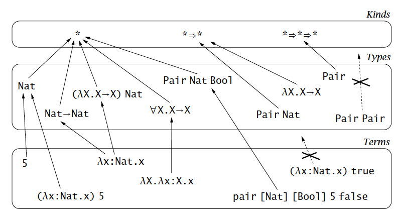
As now we can apply one type to another, it’s important to defend against meaningless expressions like “Bool Nat” just like we forbid “true 6”. This can be achieved by introducing the concept kinds, which classify type expressions according to their arity, just as arrow types tell us about the arities of terms.
*           the kind of proper types (like Bool and Bool→Bool)
*⟹*        the kind of type operators (i.e., functions from proper types
            to proper types)
*⟹*⟹*     the kind of functions from proper types to type operators
            (i.e., two-argument operators)
(*⟹*)⟹*   the kind of functions from type operators to proper types
Intuitively, kinds are “the types of types.” Following diagram illustrates the relationship among kinds, types and terms(TAPL, P444).
In theory, the hierarchy can go to infinity. But in practice, three levels is sufficient for programming languages.
The specification of higher-order polymorphic lambda calculus (Fω) is as follows:
SYNTAX

t ::=                    terms
      x                    variable
      λx:T.t               abstraction
      t t                  application
      λX ::K.t             type abstraction
      t [T]                type application

v ::=                    values
      λx:T.t               abstraction value
      λX.t                 type abstraction value

T ::=                    types
      X                    type variable
      T→T                  type of functions
      ∀X ::K .T            universal type
       λX::K.T             operator abstraction
       T T                 operator application

Γ ::=                    contexts
      ∅                    empty context
      Γ , x:T              term variable binding
      Γ , X::K             type variable binding

K ::=                    kinds
      *                    kind of proper types
      K⟹K                 kind of operators


EVALUATION

   t1  ⟶  t1'
------------------              (E-App1)
t1 t2  ⟶  t1' t2

   t2  ⟶  t2'
------------------              (E-App2)
v1 t2  ⟶  v1 t2'


(λx:T.t) v ⟶  [x ⟼ v]t         (E-AppAbs)

     t1 ⟶ t1'
-------------------             (E-TApp)
t1 [T2] ⟶ t1' [T2]

(λX::K.t) [T] ⟶  [X ⟼ T]t       (E-TappTabs)


KINDING

X::K ∈ Γ
----------                       (K-TVar)
Γ ⊢ X :: K

   Γ, X::K1 ⊢ T2::K2
-----------------------          (K-Abs)
Γ ⊢ λX::K1.T2 :: K1⟹K2

Γ ⊢ T1:: K11⟹K12    Γ ⊢ T2::K11
-------------------------------- (K-App)
      Γ ⊢ T1 T2 :: K12

Γ ⊢ T1 :: *    Γ ⊢ T2 :: *
---------------------------      (K-Arrow)
     Γ ⊢ T1→T2 :: *

Γ, X::K1 ⊢ T2 :: *
--------------------             (K-All)
Γ ⊢ ∀X::K1.T2 :: *


TYPE EQUIVALENCE

T ≡ T                            (Q-Refl)

T ≡ S
-----                            (Q-Symm)
S ≡ T

S ≡ U   U ≡ T
-------------                    (Q-Trans)
    S ≡ T

S1 ≡ T1   S2 ≡ T2
-----------------                (Q-Arrow)
  S1→S2 ≡ T1→T2

        S2 ≡ T2
-----------------------          (Q-All)
∀X::K1 .S2 ≡ ∀X::K1 .T2

       S2 ≡ T2
---------------------            (Q-Abs)
λX::K1.S2 ≡ λX::K1.T2

S1 ≡ T1    S2 ≡ T2
------------------               (Q-App)
   S1 S2 ≡ T1 T2

(λX::K11.T12) T2 ≡ [X ⟼ T2 ]T12  (Q-AppAbs)


TYPING

 x:T ∈ Γ
----------                       (T-Var)
Γ ⊢ x : T

Γ ⊢ T1::*    Γ, x:T1 ⊢ t:T2
---------------------------      (T-Abs)
    Γ ⊢ λx:T1.t : T1 → T2

Γ ⊢ t1: T → T', t2: T
-----------------------          (T-App)
  Γ ⊢ t1 t2: T

Γ, X::K ⊢ t : T
---------------------            (T-TAbs)
Γ ⊢ λX::K.t : ∀X::K.T

     Γ ⊢ t : ∀X::K.T
     Γ ⊢ T1::K
-------------------------        (T-TApp)
 Γ ⊢ t [T1] : [X ⟼ T1]T

Γ ⊢ t:S  S ≡ T   Γ ⊢ T::*
-------------------------        (T-Eq)
       Γ ⊢ t : T
Higher-Order Bounded Polymorphism
We’ve seen that kinding can be combined with System F, it’s also possible to combine kinding with System F with subtyping.
There are two important decisions to be made on how to extend bounded polymorphism with kinding:
- Whether type operators like λX::K1.T2 should be generalized to bounded type operators of the form λX<:T1.T2?
- How to extend subtype relation to include type operators?
For the first question, if bounded type operators like λX<:T1.T2 were introduced, then we’ll have to extend kinds with things like ∀X<:T1.K2, which greatly complicates the system, though it’s theoretically possible. For simplicity, here we allow type operators to be unbounded.
For the second question, the simplest solution is to lift the subtype relation on proper types point-wise to type operators. For abstractions, we say that λX.S is a subtype of λX.T whenever applying both to any argument U yields types that are in the subtype relation.
Equivalently, we can say that λX.S is a subtype of λX.T if S is a subtype of T when we hold X abstract, making no assumptions about its subtypes and supertypes.
A useful side effect of this definition is that the subtype relations for higher kinds all have maximal elements. If we let Top[*] = Top and define(maximal elements of higher kinds)
Top[K1⇒K2] = λX::K1.Top[K2],
then a simple induction shows that Γ, S::K ⊢ S <: Top[K].
The specification of higher-order bounded polymorphism is as follows:
SYNTAX

t ::=                    terms
      x                    variable
      λx:T.t               abstraction
      t t                  application
      λX <:T.t            type abstraction
      t [T]                type application

v ::=                    values
      λx:T.t               abstraction value
      λX <:T.t            type abstraction value

T ::= ...                types
      X                    type variable
      T→T                  type of functions
      ∀X <:T.T            universal type
      λX::K.T              operator abstraction
      T T                  operator application

Γ ::=                    contexts
      ∅                    empty context
      Γ , x:T              term variable binding
      Γ , X <:T            type variable binding

K ::=                    kinds
      *                    kind of proper types
      K⟹K                 kind of operators


EVALUATION

   t1  ⟶  t1'
------------------              (E-App1)
t1 t2  ⟶  t1' t2

   t2  ⟶  t2'
------------------              (E-App2)
v1 t2  ⟶  v1 t2'


(λx:T.t) v ⟶  [x ⟼ v]t         (E-AppAbs)

    t1 ⟶  t1'
-------------------             (E-TApp)
t1 [T2] ⟶  t1' [T2]

(λX <:T.t) [U] ⟶ [X ⟼ U]t       (E-TappTabs)


KINDING

Γ ⊢ Top :: *                     (K-Top)

X<:T ∈ Γ     Γ ⊢ T :: K
-------------------------        (K-TVar)
       Γ ⊢ X :: K

   Γ, X <:Top[K1] ⊢ T2::K2
-----------------------          (K-Abs)
Γ ⊢ λX::K1.T2 :: K1⟹K2

Γ ⊢ T1:: K11⟹K12    Γ ⊢ T2::K11
-------------------------------- (K-App)
      Γ ⊢ T1 T2 :: K12

Γ ⊢ T1 :: *    Γ ⊢ T2 :: *
---------------------------      (K-Arrow)
     Γ ⊢ T1→T2 :: *

Γ, X <:Top[K1] ⊢ T2 :: *
--------------------             (K-All)
Γ ⊢ ∀ <:Top[K1].T2 :: *


TYPE EQUIVALENCE

T ≡ T                            (Q-Refl)

T ≡ S
-----                            (Q-Symm)
S ≡ T

S ≡ U   U ≡ T
-------------                    (Q-Trans)
    S ≡ T

S1 ≡ T1   S2 ≡ T2
-----------------                (Q-Arrow)
  S1→S2 ≡ T1→T2

S1 ≡ T1        S2 ≡ T2
-----------------------          (Q-All)
∀X <:S1 .S2 ≡ ∀X <:T1 .T2

       S2 ≡ T2
---------------------            (Q-Abs)
λX::K1.S2 ≡ λX::K1.T2

S1 ≡ T1    S2 ≡ T2
------------------               (Q-App)
   S1 S2 ≡ T1 T2

(λX::K11.T12) T2 ≡ [X ⟼ T2]T12  (Q-AppAbs)

SUBTYPING

Γ ⊢ S<:U   Γ ⊢ U<:T   Γ ⊢ U::K
----------------------------------   (S-Trans)
     Γ ⊢ S <: T

Γ ⊢ S :: *
-------------                        (S-Top)
Γ ⊢ S <: Top

X<:T ∈ Γ
-----------                          (S-TVar)
Γ ⊢ X <: T

  Γ ⊢ T1 <: S1     Γ ⊢ S2 <: T2
----------------------------------   (S-Arrow)
     Γ ⊢ S1 → S2 <: T1 → T2


 Γ ⊢ U1::K1    Γ, X<:U1 ⊢ S2<:T2
------------------------------------ (S-All)
  Γ ⊢ ∀X<:U1.S2 <: ∀X<:U1.T2

  Γ, X<:Top[K1] ⊢ S2<:T2
---------------------------           (S-Abs)
Γ ⊢ λX::K1.S2 <: λX::K1.T2

  Γ ⊢ S1 <: T1
------------------                    (S-App)
Γ ⊢ S1 U <: T1 U

Γ ⊢ S::K    Γ ⊢ T::K    S ≡ T
-------------------------------       (S-Eq)
        Γ ⊢ S <: T


TYPING

 x:T ∈ Γ
----------                       (T-Var)
Γ ⊢ x : T

Γ ⊢ T1::*    Γ, x:T1 ⊢ t:T2
---------------------------      (T-Abs)
    Γ ⊢ λx:T1.t : T1 → T2

Γ ⊢ t1: T → T', t2: T
-----------------------          (T-App)
  Γ ⊢ t1 t2: T

Γ, X<:T ⊢ t : T
---------------------            (T-TAbs)
Γ ⊢ λX<:T.t : ∀X<:T.T

     Γ ⊢ t : ∀X<:T1.T
     Γ ⊢ T2 <: T1
-------------------------        (T-TApp)
 Γ ⊢ t [T2] : [X ⟼ T2]T

Γ ⊢  t : S    S <: T    Γ ⊢ T :: *
-----------------------------------  (T-Sub)
            Γ ⊢ t : T